OOOP thesis: Results

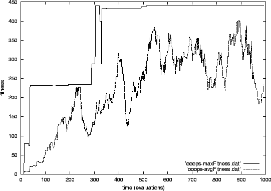
Figure 5.1 shows the development of the best fitness and the average fitness in the population during the first experiment. The optimum fitness of 441 is reached very quickly. The x-axis shows the number of evaluations and the y-axis the fitness. So if you are used to thinking in generation numbers, which is common in most evolutionary algorithms, you have to divide the value on the x-axis by the population size which in this case is 20. The optimum fitness is therefore already reached after about $\frac{300}{20}=15$ generations for the first time. And it is finally reached after about 510 evaluations which corresponds to less than 26 generations.

**Figure 5.1:** The paintable computing experiment with regular locations and ordered update.(1 generation = 20 evaluations)
$\resizebox* {1\columnwidth}{!}{\includegraphics{plot-amorphous1.eps}}$

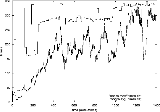
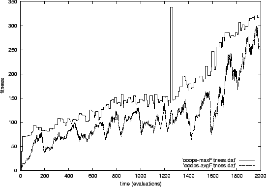
You might wonder why the best fitness sometimes decreases. The elitist approach which does not change the two best individuals should ensure not to lose the best result reached. In fact, the best individual is not lost, but it is possible that the same individual does not produce the same good results in its next evaluation. This is because there is randomness in the evaluations, for example in the initial setup. If you compare the curve of the first experiment with that of the other two runs, you see that the best fitness is much more stable in the first experiment than in the others. This is because there is much less influence of chance in the first run compared to the others: As has been described, the second and third experiment include a lot more randomness in the initial setup of the cells and the third even includes randomness in the update order.

You can see that the average fitness of the population is increasing quite steadily most of the time, but you will also notice that there are astonishingly regular periods where the average fitness heavily decreases. But this does not have any bad influence on the best fitness. In the third experiment, one even gets the impression that it sometimes helps the population to make new jumps to a better fitness level. This can perhaps be explained with the new reproduction handling introduced in OOOPS. The periods of decreasing average fitness possibly follow periods where there are no parents left in the database. The lack of parents results in many newly initialized individuals which have a high probability of getting a low fitness value. This results in the decrease of average fitness when these new individuals are evaluated. But another result of the new individuals is that totally new ideas for solving the problem can come into the population.

**Figure 5.2:** The paintable computing experiment with random locations and ordered update.(1 generation = 20 evaluations)
$\resizebox* {1\columnwidth}{!}{\includegraphics{plot-amorphous2.eps}}$

In the second experiment (shown in figure 5.2), the best fitness is very unstable (as was already explained). The average optimum fitness of 331 is already reached after approximately 190 evaluations for the first time. But it is quickly lost again. Roughly, the best fitness increases in four steps:

A level of about 40 is already reached in the randomly initialized starting population. This is easily explainable with the fact that the number of removed cells for simulating the defect reaches approximately this value. All cells in an area of $7*7$ grid points are removed which results for the second experiment in an average of $7*7*\frac{3}{4}\approx 37$ cells. So if all cells always keep the signal set, this already results in a difference of set signals of nearly 40 (and consequently a fitness with that value).

After about 100 evaluations, the best fitness reaches a level of approximately 165. This is half of the optimum fitness. It is the expected fitness if all cells set and unset their signals randomly.

After about 300 evaluations, a fitness level around 290 is reached by the best fitness curve. This level can be explained by the number of removed cells again. If no signal is set before the removal and all cells react to the defect by setting the signal, the fitness value will be equal to the number of remaining cells which is about $331-37=294$ .

The last fitness level is that of the optimum fitness which can only be reached if all cells have initially set their signals and react to the defect by unsetting it. This level is reached in the second experiment after about 1050 evaluations which corresponds to about 53 generations.

**Figure 5.3:** The paintable computing experiment with random locations and random update.(1 generation = 20 evaluations)
$\resizebox* {1\columnwidth}{!}{\includegraphics{plot-amorphous3.eps}}$

In the third experiment (shown in figure 5.3), the first best fitness reached also has a value of 40. This is (analogously to the second experiment) the case where every cell constantly keeps its signal set. But the best fitness quickly leaves this level for increasing quite slowly but constantly starting from a level of about 70. At a level of about 145, it stagnates for some time until it continues to grow after a single eye-catching peak which reaches the optimum fitness at once but loses it as quickly as it got there. Considering the relative smoothness of the rest of the curve, this peak is really astonishing. It cannot be the result of an ingenious improvement of the genome for spreading the news about the defect between the cells, because this improvement would have stayed in the population as the individual was part of the elite. Perhaps, there was a coincidence in the update order that helped in unsetting all signals. Or there was an error in the program that resulted in the removal of all cells instead of only the small block. Both explanations are not very convincing, but in any case this particularity does not seem to be important because it does not have much if any influence on the overall development of best and average fitness in the population.

The problem modelled in the third experiment seems to be much more difficult to solve than the other two. Firstly, it takes more than 2000 evaluations (or 100 generations) to reach the optimum fitness. Secondly, the best fitness curve does not stay at different levels that can be explained by simple problem solving strategies. Instead, the best fitness quite constantly (with the deviations caused by random influence) grows by improving the strategy to spread the news of the defect between the remaining cells.

**Figure 5.4:** The dynamics of the number of genes in the third experiment.(1 generation = 20 evaluations)
$\resizebox* {1\columnwidth}{!}{\includegraphics{plot-amorphous3-numGenes.eps}}$

There are some other evolutionary dynamics at which we will take a short look. We will only do this for the third experiment as it is the most interesting of the three.

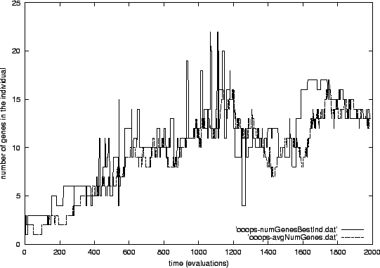
Figure 5.4 shows the development of the number of genes per individual during the evolutionary run. This graph is quite interesting, because you can see that the number of genes in the individuals slowly grows until it reaches a maximum after about 1100 evaluations. Then, it starts to vary around a number of about 13 genes until the end of the run. Though the deviations are large, it seems as if this number is a good value for ensuring the functioning of the cells. The number of genes in the best individual of the population (numGenesBestInd) is most of the time approximately equal to the average number of genes in all individuals of the population (avgNumGenes). The value of the best individual only changes more often and shows many peaks that leave the average into both directions. In most peaks however, numGenesBestInd has a higher value than avgNumGenes. This also holds for some longer periods where the two values differ from each other.

**Figure 5.5:** The dynamics of the number of commands in the evolvable code of the genes in the third experiment.(1 generation = 20 evaluations)
$\resizebox* {1\columnwidth}{!}{\includegraphics{plot-amorphous3-numCommands.eps}}$

If you look a little closer, you will notice another interesting detail: The best individual nearly always determines the direction of the development of the number of genes. When numGenesBestInd shows many peaks to higher values, the development goes towards more genes per individual. When the peaks point into the other direction, the average number of genes decreases. This can be explained by the fact, that the best individual frequently reproduces and thereby puts many new individuals into the population which contain a similar number of genes.

Another astonishing fact is, that exactly at the same time as when the fitness reaches the single eye-catching peak to the optimum, the number of genes in the best individual reaches an eye-catching peak to a low value of only four genes. This is interesting, because it seems to show that a number of about 13 genes is not really necessary for reaching the optimum fitness. Still, it is puzzling that not only the fitness of this best individual was unusual but also its number of genes shows an astonishing peak.

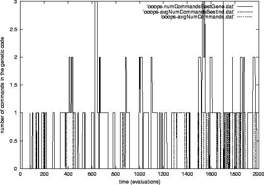
Figure 5.5 depicts the dynamics of another part of the genetic parameters during the third evolutionary run: the number of commands used in the evolvable code of the genes. This graph shows the development of three parameters: the number of commands in the best gene, the average number of commands in all genes of the best individual and the average number of commands in all genes. The only parameter that from time to time reaches a value of more than 1 is the number of commands in the best gene. This is also the only parameter that is not an average which explains its larger deviations. Even though the frequency of higher values seems to increase after about 1500 evaluations, the plot shows no real tendency of the number of commands per gene to increase. The average stays below 1 most of the time. Perhaps, the growing frequency of higher values is already a harbinger of a coming strong code elongation (called bloat in GP) after the optimum has been reached. As only the last command of a gene has any influence on the result in this setup, putting more commands into the genetic code would be a possible strategy for the individuals and genes to protect themselves against mutation².

At last, we will have a look at the "result" of the evolutionary run: the best individual. The following list shows all the variable parameters of the 18 genes of this individual. You might wonder why there are 18 genes even though figure 5.4 only showed 13 genes for the best individual at the end of the run. This is because the run was actually stopped only shortly after the 2000th evaluation. The graphs were simply cut before that for better fitting into the scales. In the following list of genes of the best individual, the first line always shows the genetic code, the second line describes the message production in the format (type, intensity) and then follow the requirements and inhibitors in the same format: